ProbabilityBench: How close are a model’s probabilities to the truth?

Why is it hard to evaluate a model’s probabilities?

We want models to make accurate predictions and to report probabilities that reflect the uncertainty of the task. This applies to ordinary classifiers like logistic regression, language models asked to estimate outcome probabilities, and decision models like Jev that return event probabilities directly. But on real-world data, we usually do not know the true probabilities, so we cannot directly check how close a model’s estimates are. A credit dataset may tell us what was known about a company and whether it later defaulted. A peer-review dataset may contain a paper’s reviews and its acceptance decision. Neither tells us the true probability of the outcome given that information.

One common approach is to check calibration: group similar predictions and compare them with observed outcome frequencies. Among companies assigned a 20% default probability, for example, do about 20% actually default? That is a useful check of the group average, but it does not establish that 20% was a good estimate for each company in the group.

Proper scoring rules such as log loss offer another approach. In expectation, log loss is uniquely minimized by reporting the true probability. In practice, we average it over a finite test set, usually with just one observed outcome per input, so the estimated score is subject to sampling error. Expected log loss also includes the uncertainty that remains even for an ideal predictor. Without knowing that contribution, the loss alone cannot tell us how much error comes from the model’s probability estimates.

The same missing information makes classification accuracy harder to interpret. The Bayes error is the lowest average classification error any predictor could achieve using the available input. The gap between a model’s error and this minimum tells us how much room for improvement remains. On real data, however, the minimum itself has to be estimated with Bayes error estimators. We then face a second evaluation problem: how do we check whether that estimate is accurate?

In simple synthetic settings, such as Gaussian mixtures with known parameters, we can derive class probabilities analytically. These settings let us test estimators against the true Bayes errors, but do not directly give us text-based tasks for language models. Datasets with repeated human annotations provide another useful reference, including for images and natural-language inference. Their label probabilities are still estimated from a finite number of annotations and can depend on how those annotations were collected. That uncertainty can make small differences between models difficult to resolve.

Building a world where we know the probabilities

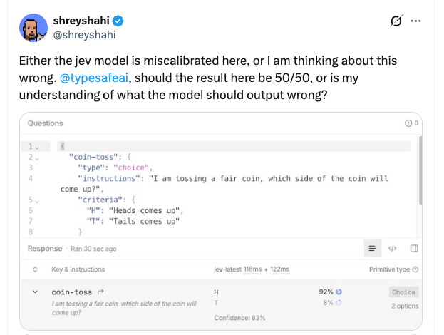
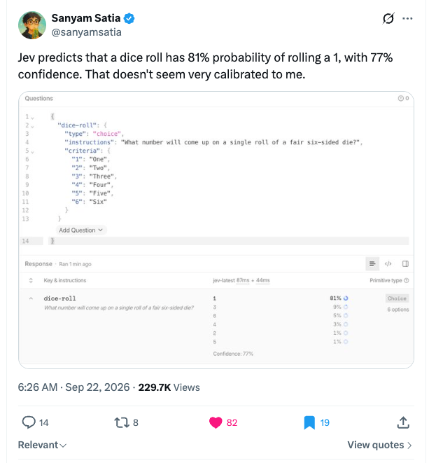
One way around this problem is to design text-based tasks whose true outcome probabilities we can compute exactly. In fact, people in the community are already exploring simple examples of this idea, such as the fair-coin and fair-die questions in the posts below. Because the prompt specifies that the coin or die is fair, we know the exact probabilities: 50% for either side of the coin and 1/6 for each face of the die. We can check a model’s estimates directly against these values.

ProbabilityBench follows the same principle, with more complex text-based worlds and an additional challenge. In our model comparison, we do not give models the full label-generating rules. They receive a small set of example texts and outcomes, then have to infer enough of the mechanism to estimate a new instance’s probability. This adds a learning problem to the probability calculation.

In ProbabilityBench, each simulated world starts with a distribution over underlying factors and a rule that determines the outcome. For each instance, models read a short text description that reveals some of those factors and withholds others. This means that several underlying situations can produce the same text but lead to different outcomes. Because we specify how the situations are generated, we can add up their probabilities to compute the exact outcome probability given the text, and the Bayes error for the world.

These are designed distributions, not models fitted to actual reviewing committees or companies. The familiar settings give the text a meaning a language model can work with, while the rules let us keep track of exactly what is knowable.

Each world has three settings, with progressively more information hidden. Their names (Low, Medium, and High) refer to the resulting Bayes error. Hiding more information raises the minimum achievable error, but it does not necessarily make the underlying rule harder to learn.

Comparing a model’s probability with the truth

Once the true probability is known, we can score a prediction without relying on the one label that happened to be drawn. We use KL divergence from the true distribution to the reported distribution. It is zero when they agree.

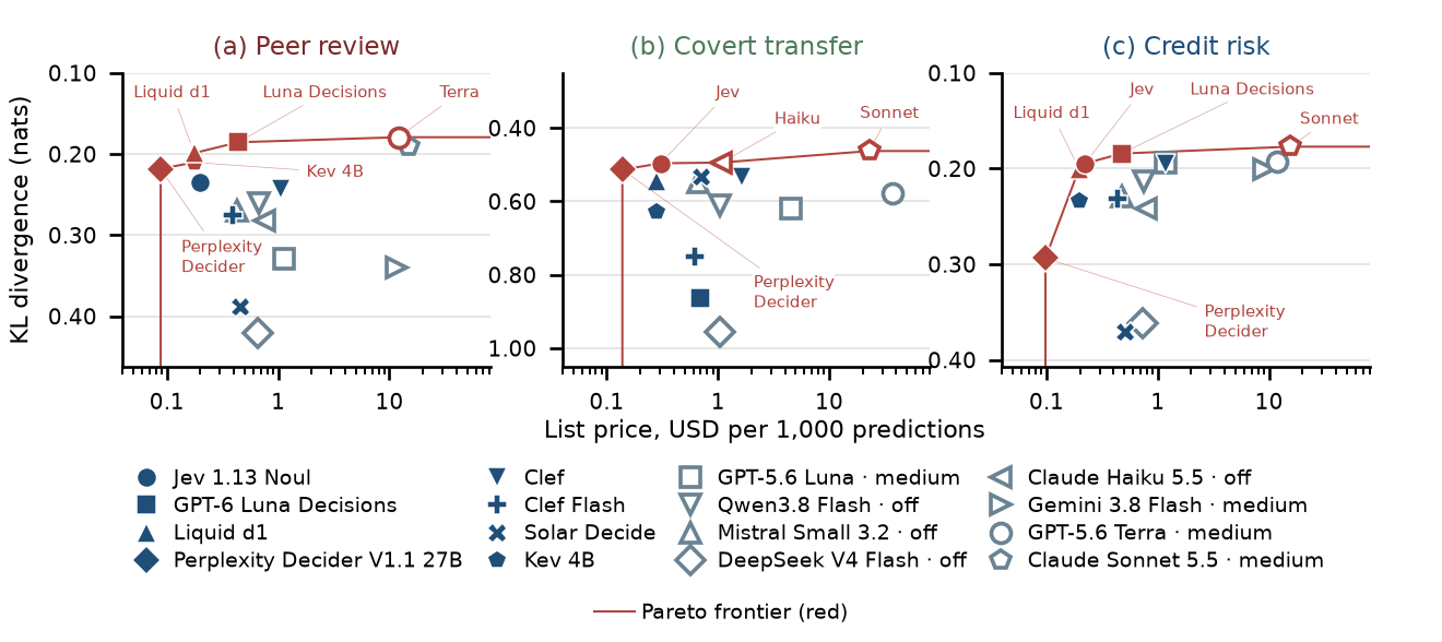
We compared eight decision models, which return event probabilities directly, and eight generative models asked to report a probability. Each received the same evidence: a text description of a test instance and 25 example descriptions paired with their observed outcomes. The comparison uses the Medium setting, with 300 test cases per world for each of three seeds. The true probabilities and hidden attributes were withheld.

In Figure 1, decision models occupy 10 of the 14 model–world points on the cost–quality frontiers. Perplexity Decider, Jev, Liquid d1, and GPT-6 Luna Decisions each appear on the Pareto frontier in at least two worlds.

Evaluation methods and agent safety

We use ProbabilityBench to check calibration metrics and Bayes-error estimators against exact reference values, a form of meta-evaluation. We also study an application of Bayes accuracy to agent safety.

• Bayes-error estimators. We test two nearest-neighbor methods against the exact Bayes error. In peer review and credit risk, their estimated intervals often lie entirely above the true value, even with 4,000 samples. The benchmark makes this overestimation of the task’s irreducible difficulty visible.
• Safety and agentic cheating. We study coding agents given access to labeled test data. Some achieve suspiciously high test accuracy by looking up answers. Their test accuracy exceeds the underlying Bayes accuracy. Reliable estimates of Bayes accuracy could help flag such results for closer inspection. We discuss related approaches to detecting test-gaming in our CapCode post and discouraging it during training in our CapReward post.
• Calibration metrics. We evaluate a multicalibration estimator using a predictor that reports the exact probabilities. We also study higher-order calibration by comparing evaluations based on repeated labels with those based on the true probabilities.

Where to go next

One direction is to explore other ways of constructing tasks with exact probabilities. We could vary the mechanisms that generate outcomes and how much information about them is given to models. Alternative designs could test kinds of probabilistic reasoning that our current three worlds do not cover.

A second direction is to make the text descriptions richer and closer to real-world text. A new renderer must preserve all visible information without revealing hidden factors. Dropping a relevant detail or adding a hint can change the probability given the text, so the exact target computed for the original attributes may no longer apply. Meeting these conditions reliably with more varied, natural descriptions is an open challenge.

We have focused on evaluation, but the same generators could also supply training data with exact probability targets. It would be interesting to study whether training decision models against these probability targets improves calibration and probability accuracy on held-out instances or new worlds.

If you’d like to learn more, our paper explains how we built the worlds and what we found. You can also find the generators and evaluation code in our repository to try the benchmark yourself or build on it.